Evolutionary Games and Population Dynamics/Well-mixed populations

In a population of varying density, an attempt at gathering \(N\) individuals that engage in a public goods interaction might not always be successful at low population densities and instead of a group of size \(N\), only \(S\leq N\) individuals participate. If \(S=0\) or \(S=1\) no interaction occurs. This leads to a natural feedback between population density and game theoretical interactions. The dynamics of cooperators and defectors in public goods interactions is determined by their respective payoffs obtained in randomly formed groups of \(S\) individuals. Independent of whether the focal individual is a cooperator or a defector, it receives the same expected payoff from its \(S-1\) co-players. Hence, the sole determinant of success is the return of the individual's own investment \(c\), which is \((r/S - 1) c\). For \(1 < r < S\) defectors are always better off as required by the traditional formulation of the public goods game. However, for \(r>S\) the social dilemma is relaxed and cooperation dominates. Nevertheless, defectors outperform cooperators in any group consisting of both types (this represents an instance of Simpson's paradox). Also note that this is a fleeting state since thriving cooperators increases the average population payoff and hence the population density which in turn leads to larger interaction groups and puts defectors back into control.
The negative feedback between population density and interaction group size hinges on the fact that the group size can become smaller than \(r\). For pairwise prisoner's dilemma interactions this is not the case: because \(S\) cannot vary (and is always equal to \(N=2\)), either \(r < S\) always holds (in which case the population goes extinct) or \(r>S\) always holds (in which case defectors disappear but cooperators persist). The dynamic feedback cannot operate in either case.
The following figures and simulations illustrate the rich dynamics of this system. For increasing \(r\) the system undergoes a series of bifurcations. A super-critical or sub-critical Hopf bifurcation gives rise to stable and unstable limit cycles, respectively, and a Bautin bifurcation may even result in a pair of stable and unstable limit cycles that collide and disappear in a saddle-node bifurcation of periodic orbits.
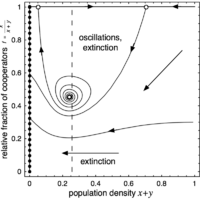
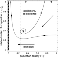
The phase space is spanned by the population density \(x + y\) (or \(1 - z\)) and the relative fraction of cooperators \(f = x / (x + y)\). The left boundary (\(z = 1\)) is attracting and consists of a line of stable fixed points (filled circles), which represent states where the population cannot maintain itself and disappears. Conversely, the right boundary, which denotes the maximal population density (\(z = 0\)), is repelling. In absence of cooperators (bottom boundary, \(f = 0\)), population densities decrease and eventually vanish. Finally, in absence of defectors (top boundary, \(f = 1\)), there are two saddle points (open circles) except for the last scenario where one is a stable node (filled circle). In addition, there may be an interior fixed point \(Q\) present.
Evolutionary scenarios
All of the following examples and suggestions are meant as inspirations for further experimenting with the EvoLudo simulator. Each of following examples starts a lab that demonstrates the particular dynamical scenario. By modifying the parameters the dynamics can be further explored.
| Color code: | Cooperators | Defectors |
|---|

(a) No Q, extinction
No matter what the initial configuration of the cooperators and defectors, the population will invariably go extinct.
Hint: start from different initial configurations to get a better intuition of the dynamics.

(b) Unstable node
The presence of the interior fixed point \(Q\) does not affect the evolutionary end state of the system - the population keeps going extinct irrespective of the initial conditions.
Hint: backwards integration reveals the location of the unstable node when starting in a suitable part of the phase plane.
(c) Unstable focus
For larger \(r\), the interior fixed point \(Q\) turns into an unstable focus and - depending on the initial conditions - the population faces extinction in an oscillatory manner.
Hint: backwards integration reveals the location of the unstable focus when starting in a suitable part of the phase plane.

Stable limit cycle - super-critical Hopf bifurcation
For slightly higher \(r\) the interior fixed point \(Q\) is still an unstable focus but now surrounded by a stable limit cycle - the hallmark of a super critical Hopf bifurcation. Cooperators and defectors co-exist in never ending periodic oscillations.
Hint: use forward and backward integration to explore the stable limit cycle and unstable fixed points.
(d) Stable focus
Increasing \(r\) further leads to a Hopf bifurcation, the interior fixed point \(Q\) becomes a stable focus and the limit cycle disappears. Depending on the initial conditions, cooperators and defectors co-exist at some fixed densities. If exploitation by defectors is severe or population densities are too low, the population is unable to recover and goes extinct.

(e) Stable node
Another increase in \(r\) turns the interior fixed point \(Q\) into a stable node. As before, cooperators and defectors co-exist at some fixed densities only, they no longer approach the equilibrium in an oscillatory manner. Severe exploitation and low population densities again result in extinction.
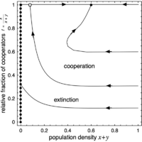
(f) No Q, cooperation
For high \(r\), the interior fixed point \(Q\) disappears and the high density saddle node along \(f=1\), i.e. in absence of defectors, becomes a stable equilibrium. Cooperators and defectors can no longer co-exist but now its only the defectors that disappear, at least for favorable initial conditions. As always, severe exploitation and low population densities result in extinction.
Complex bifurcations
For larger group sizes \(N\) fascinating and much more complex Hopf bifurcations and dynamical scenarios are possible, which includes multiple, stable and unstable limit cycles. However, also note that r values for which these fascinating bifurcations occur is restricted to a tiny interval. Thus, despite their appeal from a dynamical systems' perspective, the limit cycles might be of only limited relevance for biological applications.
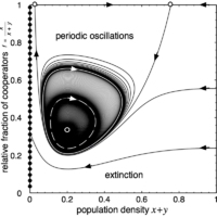
Multiple limit cycles - Bautin bifurcation
In this example, for \(N=12\), a stable and an unstable limit cycle exist on one side of the Hopf bifurcation and another stable limit cycle on the other side.
Hint: Try lowering \(r\) slightly to just below the Hopf-bifurcation (set \(r = 3.04\)). The interior fixed point \(Q\) is now an unstable focus surrounded by a stable limit cycle (see above).

Unstable limit cycle - sub-critical Hopf bifurcation
In the special case \(b=0\) sub-critical Hopf-bifurcations always seem to give rise to a pair of stable and unstable limit cycles (Bautin bifurcation). Apparently only for \(b>0\) a simple sub-critical Hopf-bifurcation can be observed.
Population Dynamics
In order to combine game dynamics and population dynamics in a replicator equation we assume that \(u\) denotes the density of cooperators, \(v\) the density of defectors and \(w=1-u-v\) represents a measure for reproductive opportunities such as the abundance of food or availability of space. Thus, \(u+v\) denotes a normalized population density such that for \(u+v=0\) (or \(w=1\)) the population has gone extinct. The dynamics of \(u, v\) and \(z\) is determined by the average payoffs (or fitness) of cooperators \(f_C\) and defectors \(f_D\) arising from game theoretical interactions. Cooperators and defectors are assumed to die at a constant rate \(d\) and give birth according to a constant baseline birth rate \(b\) augmented by their performance \(f_C\) and \(f_D\). In addition, birth events are conditional on the availability of empty space and hence are proportional to \(w\). This leads to the following population dynamic model:
\begin{align*} \dot u =& u (w (b+f_C)-d)\\ \dot v =& v (w (b+f_D)-d)\\ \dot w =& -\dot u -\dot v \end{align*}
This system of equations represents a natural extension of the replicator dynamics. If the population density \(u+v\) is kept constant (\(\dot w = 0\)) by adjusting the death rate accordingly, i.e. by setting \(d = w(b+\bar f/(1-w))\), where \(\bar f = u\ f_C+v\ f_D\) denotes the mean fitness, the traditional replicator dynamics is recovered (upon normalizing \(u+v=1\)). The average payoffs \(f_C\) and \(f_D\) are determined by the actual game theoretical interactions under consideration.