Moran graphs

Author: Christoph Hauert

Fairly generic sample population structure. Vertices represent individuals and links define their neighbourhood. A directed link indicates that one individual may be another's neighbour but not vice versa. Each link may have a weight, which indicates the propensity to be selected for reproduction. Reproduction occurs in the direction of the link. The depicted graph represents a circulation and hence a mutant has the same fixation probability as in the original Moran process for unstructured populations.

Moran graphs maintain the balance between selection and random drift of the original Moran process. For those graphs the spatial Moran process leaves the fixation probabilities of a mutant unchanged and identical to the original Moran process in unstructured, well-mixed populations. Rather surprisingly it turns out that this applies to a large class of graphs, called circulations.

Mathematically, the structure of the graph is determined by the adjacency matrix \(\mathbf{W} = [w_{ij}]\) where \(w_{ij}\) denotes the strength of the link pointing from vertex \(i\) to vertex \(j\). If \(w_{ij} =0\) and \(w_{ji} =0\) then the two vertices \(i\) and \(j\) are not connected. In order to characterize circulations, let us introduce the flux through each vertex. The sum of the weights of the incoming links \(f_i^\text{in}=\sum_j w_{ji}\) denotes the flux entering vertex \(i\). \(f_i^\text{in}\) relates to a temperature because it indicates the rate at which the occupant of vertex \(i\) gets replaced. ‘Hot’ vertices are frequently replaced and ‘cold’ vertices are only rarely updated. In analogy, the sum of the weights of the outgoing links \(f_i^\text{out}=\sum_j w_{ij}\) denotes the flux leaving vertex \(i\). \(f_i^\text{out}\) determines the impact of vertex \(i\) on its neighborhood. All graphs, which satisfy \(f_i^\text{in}=f_i^\text{out}\) for all vertices, are circulations. With this we can state a remarkable theorem:

Circulation Theorem: The Moran process on a graph results in the same fixation probability \(\rho_1\) of a single mutant as in an unstructured population if the graph is a circulation.

An illustrative sketch of the proof follows below. In contrast to unstructured (well-mixed) populations, the state of a structured population is not simply determined by just the number of mutants (or residents) but rather needs to take the distribution of mutants and residents into account. Rather surprisingly, however, it turns out that for circulations the spatial distribution of mutants and residents does not affect their fixation probabilities. The observation that fixation probabilities remain unchanged for diverse population structures forms the basis for the conjecture by Maruyama (1970) and Slatkin (1981) speculating that population structure does not affect fixation probabilities. Indeed this is true for structures as diverse as complete graphs (every vertex is connected to every other vertex), lattices or random regular graphs (see e.g. Bollobás, 1995).

Last but not least, the circulation theorem indirectly suggests that some population structures do affect fixation probabilities. Thus, it becomes an intriguing question what population structures may act as evolutionary suppressors that suppress selection and enhance random drift (\(\rho<\rho_1\) for \(r > 1\)) or, conversely, as evolutionary amplifiers that enhance selection and suppresses random drift (\(\rho>\rho_1\) for \(r > 1\)).

Evolutionary dynamics on Moran graphs

Evolutionary dynamics on the complete graph

.

Evolutionary dynamics on the linear graph

.

Evolutionary dynamics on the rectangular lattice

.

Evolutionary dynamics on random regular graphs

.

Fixation probabilities on Moran graphs

Fixation probabilities on the complete graph

.

Fixation probabilities on the linear graph

.

Fixation probabilities on the rectangular lattice

.

Fixation probabilities on random regular graphs

.

Fixation times on Moran graphs

Fixation times on the complete graph

.

Fixation times on the linear graph

.

Fixation times on the rectangular lattice

.

Fixation times on random regular graphs

.

Fixation probability on circulation graphs

Circulation graph with one connected subset (shaded area) of mutants (orange). For every reproduction event along one of the solid arrows, the subset either shrinks, if a resident (blue) reproduced, or grows, if a mutant reproduces. Reproduction events along dashed arrows do not alter the population configuration.

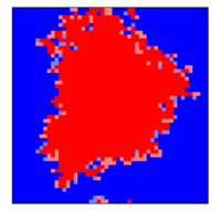
At any point in time during the invasion process of mutants on a circulation graph, it is possible to identify connected subsets of vertices on the graph that are occupied by mutants such that all adjacent vertices of each subset are occupied by residents. Obviously, the state of the population changes only if a replacement occurs along one of the links connecting residents and mutants (see figure). Multiple such subsets may exist and, in fact, the evolutionary process may split large connected subsets of mutants into two smaller ones or may merge two previously unconnected subsets into one larger subset. For each subset, the circulation theorem establishes that the sum of the weights of links pointing out of the subset (connecting a mutant vertex to an adjacent resident vertex) equals the sum of the weights of links pointing into the subset (connecting an adjacent resident with a mutant vertex within the subset). Since the influx is balanced by the outflux, \(f_i^\text{in}=f_i^\text{out}\), for all vertices, increasing the mutant subset by replacing an adjacent resident vertex with a mutant or decreasing the subset by replacing a mutant with a resident, does not affect the flux balance of the subset. For the same reason, the balance remains unchanged if subsets merge or if one subset splits into two.

Recall that the number of mutants in the population changes only if a replacement occurs along any link that connects residents with mutants or vice versa. Because the Moran process essentially selects links with a probability proportional to the link weight and the fitness of the vertex at its tail, it follows that for each subset, the probability that another mutant is added is simply given by \(r/(1 + r)\) and the complementary probability to remove one mutant is \(1/(1 + r)\). Since this holds for each subset, it also holds for the entire population and is independent of the number, size, shape and distribution of mutant subsets. This invariance applies only if the circulation theorem is satisfied. Consequentially, the fixation probability on circulation graphs reduces to the recursive equation derived for the original Moran process.

Note that even though the fixation probabilities remain unchanged on circulation graphs, the corresponding fixation times are very sensitive to the details of the population structure and pose a much harder problem. The circulation theorem only ensures that the ratio of the transition probabilities \(T^+/T^− = r\) remains unchanged, i.e. independent of the number and distribution of residents and mutants, but even on circulation graphs \(T^+\) and \(T^−\) depend not only on the number but also on the distribution of mutants. Generally, population structures tend to substantially increase the fixation times because the structure limits the possibilities for mutants to conquer new vertices.

Publications

1. Lieberman, E., Hauert, C. & Nowak, M. (2005) Evolutionary dynamics on graphs Nature 433 312-316 doi: 10.1038/nature03204.

References

1. Bollobás, B. (1995) Random Graphs, New York, Academic.
2. Maruyama, T. (1974) A Simple Proof that Certain Quantities are Independent of the Geographical Structure of Population Theor. Pop. Biol. 5 148-154.
3. Slatkin, M. (1981) Fixation probabilities and fixation times in a subdivided population Evolution 35 477-488.