Stochastic dynamics in finite populations: Difference between revisions
| (8 intermediate revisions by the same user not shown) | |||
| Line 1: | Line 1: | ||
{{InCharge|author1=Christoph Hauert}} | |||
{{TOCright}} | {{TOCright}} | ||
Stochastic differential equations (SDE) provide a general framework to describe the evolutionary dynamics of an arbitrary number of types in finite populations, which results in demographic noise, | Stochastic differential equations (SDE) provide a general framework to describe the evolutionary dynamics of an arbitrary number of strategic types \(d\) in finite populations, which results in demographic noise, as well as to incorporate mutations. For large, but finite populations this allows to include demographic noise without requiring explicit simulations. Instead, the population size only rescales the amplitude of the noise. Moreover, this framework admits the inclusion of mutations between different types, provided that mutation rates, \(\mu\), are not too small compared to the inverse population size \(1/N\). This ensures that all types are almost always represented in the population and that the occasional extinction of one type does not result in an extended absence of that type. For \(\mu N\ll1\) this limits the use of SDE’s, but in this case well established alternative approximations are available based on time scale separation. | ||
The tutorial on [[2×2_Games/Stochastic_dynamics|stochastic dynamics in \(2\times2\) games]] covers the simpler case with two strategic types, \(d=2\). Here we focus on the general case with \(d>2\) strategic types and illustrate our approach based on the [[Rock-Scissors-Paper game]] with mutations (\(d=3\)). The stochastic dynamics is in excellent agreement with simulation based results for sufficiently large populations. In the absence of mutations the excellent agreement extends to small population sizes. | |||
''This tutorial complements a series of [[#References|research articles]] by [http://www.evolbio.mpg.de/~traulsen/ Arne Traulsen], [http://www.inb.uni-luebeck.de/~claussen/ Jens Christian Claussen] & [http://www.math.ubc.ca/~hauert/ Christoph Hauert]'' | ''This tutorial complements a series of [[#References|research articles]] by [http://www.evolbio.mpg.de/~traulsen/ Arne Traulsen], [http://www.inb.uni-luebeck.de/~claussen/ Jens Christian Claussen] & [http://www.math.ubc.ca/~hauert/ Christoph Hauert]'' | ||
| Line 7: | Line 10: | ||
==Rock-Paper-Scissors game== | ==Rock-Paper-Scissors game== | ||
[[Image:Stochastic dynamics - noise term Cxx, no mutations.png|300px|thumb| | [[Image:Stochastic dynamics - noise term Cxx, no mutations.png|300px|thumb|Demographic noise in evolutionary dynamics with \(d = 3\) strategic types in the absence of mutations, \(\mu = 0\). The value of the element \(\mathcal C_{xx}(x,y,z)\) of the noise matrix \(\mathcal C(\mathbf x)\) is shown. \(\mathcal C_{xx}(x,y,z)\) determines how the noise in the \(x\)-direction affects the \(x\)-coordinate. In the case of \(\mu = 0\), this noise vanishes for \(x\to0\). For \(y\to0\) and \(z\to0\) we recover the usual multiplicative noise from one-dimensional evolutionary processes.]] | ||
The [[Rock-Paper-Scissors game]] exhibits cyclic dominance among its three strategic types: Rock beats Scissors beats Paper beats Rocks etc. In evolving populations this gives rise to oscillations in the abundance of each strategic type. The amplitude of these oscillation may (i) decrease over time resulting in stable equilibrium frequencies, (ii) keep increasing and approaching a heteroclinic cycle along the boundary of the simplex \(S_3\) or result in the extinction of one type and eventual reach an absorbing homogenous state or, (iii) give rise to stable limit cycles. | |||
Comparisons between the deterministic dynamics in infinite populations, the stochastic dynamics in finite populations and individual based simulations | Comparisons between the deterministic dynamics in infinite populations, the stochastic dynamics in finite populations and individual based simulations are illustrated for a generic payoff matrix | ||
\[\begin{matrix}~&\begin{matrix}\ \ R\quad & S\quad & P\quad\end{matrix} \\ | |||
\begin{matrix}R\\S\\P\end{matrix}& | \begin{matrix}R\\S\\P\end{matrix}& | ||
\begin{pmatrix}0 & \frac{s}{2} & -1 \\ | \begin{pmatrix}0 & {\textstyle\frac{s}{2}} & -1 \\ | ||
-1 & 0 & 2+s \\ | -1 & 0 & 2+s \\ | ||
\frac{1+s}{3} & -1 & 0\end{pmatrix}\end{matrix}. | {\textstyle\frac{1+s}{3}} & -1 & 0\end{pmatrix}\end{matrix}. | ||
\] | |||
According to the [[replicator equation]] the game exhibits saddle node fixed points at | According to the [[replicator equation]] the game exhibits saddle node fixed points at \(x = 1, y = 1\), and \(z = 1-x-y = 1\) as well as an interior fixed point at \(\textstyle\hat{\mathbf x} = \left(\frac12,\frac13,\frac16\right)\) independent of the parameter \(s\). For \(s > 1\), \(\hat x\) is a stable focus and an unstable focus for \(s < 1\). In the non-generic case \(s=1\) the dynamics exhibits closed orbits. | ||
{{-}} | {{-}} | ||
| Line 25: | Line 30: | ||
[[Image:RSP - ODE.svg|left|200px|link=EvoLudoLab: Rock-Paper-Scissors - ODE]] | [[Image:RSP - ODE.svg|left|200px|link=EvoLudoLab: Rock-Paper-Scissors - ODE]] | ||
====[[EvoLudoLab: Rock-Paper-Scissors - ODE|Replicator dynamics - Attractor]]==== | ====[[EvoLudoLab: Rock-Paper-Scissors - ODE|Replicator dynamics - Attractor]]==== | ||
In the limit | In the limit \(N\to\infty\) demographic stochasticity arising in finite populations disappears and the dynamics becomes deterministic. For \(s>1\) the interior fixed point \(\hat x\) is a stable focus of the replicator dynamics. All trajectories spiral toward \(\hat x\). | ||
{{-}} | {{-}} | ||
</div> | </div> | ||
| Line 33: | Line 38: | ||
==== [[EvoLudoLab: Rock-Paper-Scissors - ODE with Mutations|Replicator-Mutator dynamics - Stable limit cycle]]==== | ==== [[EvoLudoLab: Rock-Paper-Scissors - ODE with Mutations|Replicator-Mutator dynamics - Stable limit cycle]]==== | ||
For | For \(s < 1\) the interior fixed point \(\hat x\) is an unstable focus. The trajectories spiral away from \(\hat x\) and, in the absence of mutations, approach the heteroclinic cycle along the boundary of the simplex \(S_3\). With mutation rates \(\mu>0\), however, the boundary of \(S_3\) becomes repelling, which can give rise to stable limit cycles. If the mutation rate is sufficiently high, the interior fixed point is stable again. The image shows a sample trajectory for \(s=0.2\), \(\mu=0.001\). | ||
{{-}} | {{-}} | ||
</div> | </div> | ||
| Line 41: | Line 46: | ||
[[Image:RSP - SDE.svg|left|200px|link=EvoLudoLab: Rock-Paper-Scissors - SDE]] | [[Image:RSP - SDE.svg|left|200px|link=EvoLudoLab: Rock-Paper-Scissors - SDE]] | ||
==== [[EvoLudoLab: Rock-Paper-Scissors - SDE|Stochastic differential equations]]==== | ==== [[EvoLudoLab: Rock-Paper-Scissors - SDE|Stochastic differential equations]]==== | ||
The interior fixed point \(\hat x\) is a stable focus of the replicator dynamics, \(s < 1\). Demographic stochasticity arises from the finite population size of \(N = 100\). In the absence of mutations, the boundaries remain absorbing and even though the interior fixed point is attracting, stochastic fluctuations nevertheless eventually drive the population to the absorbing boundaries. | |||
{{-}} | {{-}} | ||
</div> | </div> | ||
| Line 47: | Line 53: | ||
[[Image:RSP - SDE Mutations.svg|left|200px|link=EvoLudoLab: Rock-Paper-Scissors - SDE with Mutations]] | [[Image:RSP - SDE Mutations.svg|left|200px|link=EvoLudoLab: Rock-Paper-Scissors - SDE with Mutations]] | ||
==== [[EvoLudoLab: Rock-Paper-Scissors - SDE with Mutations|Stochastic differential equations, with mutations]]==== | ==== [[EvoLudoLab: Rock-Paper-Scissors - SDE with Mutations|Stochastic differential equations, with mutations]]==== | ||
The interior fixed point \(\hat x\) of the replicator dynamics is an unstable focus. Even without stochasticity all trajectories spiral away from \(\hat x\) toward the boundary of the simplex \(S_3\). However, due to mutations, the boundary is repelling, which results in a stochastic analog of a stable limit cycle. For larger mutation rates the interior fixed point becomes stable again even for \(s<1\). | |||
{{-}} | {{-}} | ||
</div> | </div> | ||
| Line 54: | Line 61: | ||
[[Image:RSP - IBS.svg|left|200px|link=EvoLudoLab: Rock-Paper-Scissors - IBS]] | [[Image:RSP - IBS.svg|left|200px|link=EvoLudoLab: Rock-Paper-Scissors - IBS]] | ||
==== [[EvoLudoLab: Rock-Paper-Scissors - IBS|Individual based simulations]]==== | ==== [[EvoLudoLab: Rock-Paper-Scissors - IBS|Individual based simulations]]==== | ||
The interior fixed point \(\hat x\) is a stable focus of the replicator dynamics. Stochastic fluctuations arise in individual based simulations of populations with a finite size, \(N=1000\). In the absence of mutations, the boundaries are absorbing and even though the interior fixed point is attracting, the population will eventually end up in one of the absorbing homogenous states with all rock, all paper or all scissors. | |||
{{-}} | {{-}} | ||
</div> | </div> | ||
| Line 60: | Line 68: | ||
[[Image:RSP - IBS Mutations.svg|left|200px|link=EvoLudoLab: Rock-Paper-Scissors - IBS with Mutations]] | [[Image:RSP - IBS Mutations.svg|left|200px|link=EvoLudoLab: Rock-Paper-Scissors - IBS with Mutations]] | ||
==== [[EvoLudoLab: Rock-Paper-Scissors - IBS with Mutations|Individual based simulations, with mutations]]==== | ==== [[EvoLudoLab: Rock-Paper-Scissors - IBS with Mutations|Individual based simulations, with mutations]]==== | ||
The interior fixed point \(\hat x\) of the replicator dynamics is an unstable focus. Even without stochasticity all trajectories spiral away from \(\hat x\) towards the boundary of the simplex \(S_3\). However, due to mutations, the boundary is repelling, which results in a stochastic analog of a stable limit cycle. Larger mutation rates increasingly limit the range of values that can be attained by the mean frequencies of the three strategies. In particular, in the limit \(\mu\to1\) the game payoffs no longer affect the dynamics and the mean of all three strategies is simply \(1/3\). | |||
{{-}} | {{-}} | ||
</div> | </div> | ||
==From finite to infinite populations== | ==From finite to infinite populations== | ||
[[Image:SDE vs IBS Performance.svg|300px|thumb|Performance comparison of individual based simulations (IBS) versus stochastic differential equations (SDE). '''a''' ratio of the CPU times | [[Image:SDE vs IBS Performance.svg|300px|thumb|Performance comparison of individual based simulations (IBS) versus stochastic differential equations (SDE). '''a''' ratio of the CPU times \(CPU_\text{SDE}/CPU_\text{IBS}\) as a function of the population size, \(N\), and the number of strategic types, \(d\). The bold contour indicates equal performance. | ||
For small | For small \(N\) and large \(d\) IBS are faster (red region), but for larger \(N\) and smaller \(d\) SDE are faster (blue region). | ||
Each contour indicates a performance difference of one order of magnitude. | Each contour indicates a performance difference of one order of magnitude. | ||
'''b''' computational time with | '''b''' computational time with \(d=10\) as a function of \(N\) for IBD (red) and SDE (blue). As a reference for the scaling \(N^2\) (red) and a constant (blue) are shown. '''c''' computational time with \(N=5000\) as a function of \(d\) for IBD (red) and SDE (blue). As a reference for the scaling \(d^{1/2}\) (red) and \(d^3\) (blue) are shown. For a proper scaling argument much larger \(d\) are required but already \(d=100\) far exceeds typical evolutionary models and hence is only of limited relevance in the current context. All comparisons use a constant payoff matrix and the local update process (such that \({\mathcal A}_k(\mathbf x)=0\) and \(\gamma(\pi_j, \pi_k)=1/2\)), a mutation rate of \(1/N\) and are based on at least \(1000\) time steps as well as at least one minute running time. CPU time is measured in milliseconds required to calculate \(1000\) time steps. The time increment for the SDE is \(dt=0.01\).]] | ||
In unstructured, finite populations of constant size, | In unstructured, finite populations of constant size, \(N\), consisting of \(d\) distinct strategic types and with a mutation rate, \(\mu\), evolutionary changes can be described by the following class of birth-death processes: In each time step, one individual of type \(j\) produces a single offspring and displaces another randomly selected individual of type \(k\). With probability \(1-\mu\), no mutation occurs and \(j\) produces an offspring of the same type. But with probability \(\mu\), the offspring of an individual of type \(i\) (\(i\neq j\)) mutates into a type \(j\) individual. This results in two distinct ways to increase the number of \(j\) types by one at the expense of decreasing the number of \(k\) types by one, hence keeping the population size constant. Biologically, keeping \(N\) constant implies that the population has reached a stable ecological equilibrium and assumes that this equilibrium remains unaffected by trait frequencies. The probability for the event of replacing a type \(k\) individual with a type \(j\) individual is denoted by \(T_{kj}\) and is a function of the state of the population \(\mathbf X=(X_1, X_2, \ldots X_d)\), with \(X_n\) indicating the number of individuals of type \(n\) such that \(\textstyle\sum_{n=1}^d X_n = N\). | ||
For such processes we can easily derive a Master equation: | For such processes we can easily derive a Master equation: | ||
\begin{equation*} | |||
P^{\tau+1}({\mathbf X}) = P^{\tau}({\mathbf X})+\!\sum_{j,k=1}^d\! P^{\tau}({\mathbf X}_j^k) T_{kj}({\mathbf X}_j^k)-P^{\tau}({\mathbf X})\ T_{jk}({\mathbf X})) | |||
\end{equation*} | |||
where | where \(P^\tau({\mathbf X})\) denotes the probability of being in state \(\mathbf X\) at time \(\tau\) and \({\mathbf X}_j^k=(X_1, \ldots X_j-1, \ldots X_k+1, \ldots X_d)\) represents a state adjacent to \(\mathbf X\). For large but finite \(N\) the Kramers-Moyal expansion yields a convenient approximation in the form of a Fokker-Planck equation: | ||
\begin{align*} | |||
\dot \rho({\mathbf x}) = -\sum_{k=1}^{d-1}\frac{\partial}{\partial x_k}\rho({\mathbf x}){\mathcal A}_{k}({\mathbf x})+\frac12\sum_{j,k=1}^{d-1}\frac{\partial^2}{\partial x_k\partial x_j}\rho({\mathbf x}){\mathcal B}_{jk}({\mathbf x}) | |||
\end{align*} | |||
where | where \({\mathbf x} = {\mathbf X}/N\) represents the state of the population in terms of frequencies of the different strategic types and \(\rho({\mathbf x})\) is the probability density in state \(\mathbf x\). The drift vector \({\mathcal A}_{k}({\mathbf x})\) is given by | ||
\begin{align*} | |||
{\mathcal A}_{k}({\mathbf x}) = \sum_{j=1}^{d} \Big(T_{j k}({\mathbf x}) - T_{k j}({\mathbf x}) \Big) = -1+\sum_{j=1}^{d} T_{j k}({\mathbf x}) | |||
\end{align*} | |||
For the second equality we have used | For the second equality we have used \(\textstyle\sum_{j=1}^d T_{kj}({\boldsymbol x})=1\), which simply states that a \(k\)-type individual transitions to some other type (including staying type \(k\)) with probability one. \({\mathcal A}_{k}({\mathbf x})\) is bounded in \([-1, d-1]\) because the \(T_{jk}\) are probabilities. | ||
The diffusion matrix | The diffusion matrix \({\mathcal B}_{jk}({\mathbf x})\) is defined as | ||
\begin{align*} | |||
{\mathcal B}_{jj}({\mathbf x}) &= \frac{1}{N} \sum_{l=1,l\neq j}^d \Big(T_{j l}({\mathbf x})+T_{l j}({\mathbf x}) \Big)\end{align} | {\mathcal B}_{jk}({\mathbf x}) &= - \frac{1}{N} \left[ T_{j k}({\mathbf x}) + T_{k j}({\mathbf x}) \right] \quad {\rm for} \quad j \neq k \\ | ||
{\mathcal B}_{jj}({\mathbf x}) &= \frac{1}{N} \sum_{l=1,l\neq j}^d \Big(T_{j l}({\mathbf x})+T_{l j}({\mathbf x}) \Big) | |||
\end{align*} | |||
Note that the diffusion matrix is symmetric, | Note that the diffusion matrix is symmetric, \({\mathcal B}_{jk}({\mathbf x}) = {\mathcal B}_{kj}({\mathbf x})\) and vanishes as \(\sim 1/N\) in the limit \(N\to\infty\). | ||
The noise arising through demographic changes and mutations is uncorrelated in time and hence the Itô calculus can be applied to derive a Langevin equation | The noise arising through demographic changes and mutations is uncorrelated in time and hence the Itô calculus can be applied to derive a Langevin equation | ||
\begin{align*} | |||
\dot x_k = {\mathcal A}_k({\mathbf x}) + \sum_{j=1}^{d-1} {{\mathcal C}_{kj}({\mathbf x})} \xi_j(t) \end{align*} | |||
where the \(\xi_j(t)\) represent uncorrelated Gaussian white noise with unit variance, \(\langle \xi_k(t) \xi_j(t^\prime) \rangle = \delta_{kj} \delta(t-t^\prime)\). The matrix \({{\mathcal C}({\mathbf x})}\) is defined by \({\mathcal C}^T({\mathbf x}) {\mathcal C}({\mathbf x}) = {\mathcal B}({\mathbf x})\) and its off-diagonal elements are responsible for correlations in the noise of different strategic types. In the limit \(N\to\infty\) the matrix \({\mathcal C}({\mathbf x})\) vanishes with \(\sim 1/\sqrt{N}\) and we recover a deterministic replicator mutator equation. | |||
==References== | ==References== | ||
# Traulsen, A., Claussen, J. C. & Hauert, C. (2012) Stochastic differential equations for evolutionary dynamics with demographic noise and mutations. ''Phys. Rev. E'' | # Traulsen, A., Claussen, J. C. & Hauert, C. (2012) Stochastic differential equations for evolutionary dynamics with demographic noise and mutations. ''Phys. Rev. E'' '''85''' 041901 [http://dx.doi.org/10.1103/PhysRevE.85.041901 doi: 10.1103/PhysRevE.85.041901]. | ||
# Traulsen, A., Claussen, J. C. & Hauert, C. (2006) Coevolutionary dynamics in large, but finite populations. ''Phys. Rev. E'' '''74''' 011901 [http://dx.doi.org/10.1103/PhysRevE.74.011901 doi: 10.1103/PhysRevE.74.011901]. | # Traulsen, A., Claussen, J. C. & Hauert, C. (2006) Coevolutionary dynamics in large, but finite populations. ''Phys. Rev. E'' '''74''' 011901 [http://dx.doi.org/10.1103/PhysRevE.74.011901 doi: 10.1103/PhysRevE.74.011901]. | ||
# Traulsen, A., Claussen, J. C. & Hauert, C. (2005) Coevolutionary Dynamics: From Finite to Infinite Populations. ''Phys. Rev. Lett.'' '''95''' 238701 [http://dx.doi.org/10.1103/PhysRevLett.95.238701 doi: 10.1103/PhysRevLett.95.238701]. | # Traulsen, A., Claussen, J. C. & Hauert, C. (2005) Coevolutionary Dynamics: From Finite to Infinite Populations. ''Phys. Rev. Lett.'' '''95''' 238701 [http://dx.doi.org/10.1103/PhysRevLett.95.238701 doi: 10.1103/PhysRevLett.95.238701]. | ||
[[Category:Tutorial]] | |||
Revision as of 22:23, 3 April 2012
Stochastic differential equations (SDE) provide a general framework to describe the evolutionary dynamics of an arbitrary number of strategic types \(d\) in finite populations, which results in demographic noise, as well as to incorporate mutations. For large, but finite populations this allows to include demographic noise without requiring explicit simulations. Instead, the population size only rescales the amplitude of the noise. Moreover, this framework admits the inclusion of mutations between different types, provided that mutation rates, \(\mu\), are not too small compared to the inverse population size \(1/N\). This ensures that all types are almost always represented in the population and that the occasional extinction of one type does not result in an extended absence of that type. For \(\mu N\ll1\) this limits the use of SDE’s, but in this case well established alternative approximations are available based on time scale separation.
The tutorial on stochastic dynamics in \(2\times2\) games covers the simpler case with two strategic types, \(d=2\). Here we focus on the general case with \(d>2\) strategic types and illustrate our approach based on the Rock-Scissors-Paper game with mutations (\(d=3\)). The stochastic dynamics is in excellent agreement with simulation based results for sufficiently large populations. In the absence of mutations the excellent agreement extends to small population sizes.
This tutorial complements a series of research articles by Arne Traulsen, Jens Christian Claussen & Christoph Hauert
Rock-Paper-Scissors game

The Rock-Paper-Scissors game exhibits cyclic dominance among its three strategic types: Rock beats Scissors beats Paper beats Rocks etc. In evolving populations this gives rise to oscillations in the abundance of each strategic type. The amplitude of these oscillation may (i) decrease over time resulting in stable equilibrium frequencies, (ii) keep increasing and approaching a heteroclinic cycle along the boundary of the simplex \(S_3\) or result in the extinction of one type and eventual reach an absorbing homogenous state or, (iii) give rise to stable limit cycles.
Comparisons between the deterministic dynamics in infinite populations, the stochastic dynamics in finite populations and individual based simulations are illustrated for a generic payoff matrix
\[\begin{matrix}~&\begin{matrix}\ \ R\quad & S\quad & P\quad\end{matrix} \\ \begin{matrix}R\\S\\P\end{matrix}& \begin{pmatrix}0 & {\textstyle\frac{s}{2}} & -1 \\ -1 & 0 & 2+s \\ {\textstyle\frac{1+s}{3}} & -1 & 0\end{pmatrix}\end{matrix}. \]
According to the replicator equation the game exhibits saddle node fixed points at \(x = 1, y = 1\), and \(z = 1-x-y = 1\) as well as an interior fixed point at \(\textstyle\hat{\mathbf x} = \left(\frac12,\frac13,\frac16\right)\) independent of the parameter \(s\). For \(s > 1\), \(\hat x\) is a stable focus and an unstable focus for \(s < 1\). In the non-generic case \(s=1\) the dynamics exhibits closed orbits.
Deterministic Dynamics

Replicator dynamics - Attractor
In the limit \(N\to\infty\) demographic stochasticity arising in finite populations disappears and the dynamics becomes deterministic. For \(s>1\) the interior fixed point \(\hat x\) is a stable focus of the replicator dynamics. All trajectories spiral toward \(\hat x\).
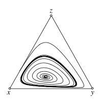
Replicator-Mutator dynamics - Stable limit cycle
For \(s < 1\) the interior fixed point \(\hat x\) is an unstable focus. The trajectories spiral away from \(\hat x\) and, in the absence of mutations, approach the heteroclinic cycle along the boundary of the simplex \(S_3\). With mutation rates \(\mu>0\), however, the boundary of \(S_3\) becomes repelling, which can give rise to stable limit cycles. If the mutation rate is sufficiently high, the interior fixed point is stable again. The image shows a sample trajectory for \(s=0.2\), \(\mu=0.001\).
Stochastic Dynamics
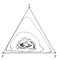
Stochastic differential equations
The interior fixed point \(\hat x\) is a stable focus of the replicator dynamics, \(s < 1\). Demographic stochasticity arises from the finite population size of \(N = 100\). In the absence of mutations, the boundaries remain absorbing and even though the interior fixed point is attracting, stochastic fluctuations nevertheless eventually drive the population to the absorbing boundaries.
Stochastic differential equations, with mutations
The interior fixed point \(\hat x\) of the replicator dynamics is an unstable focus. Even without stochasticity all trajectories spiral away from \(\hat x\) toward the boundary of the simplex \(S_3\). However, due to mutations, the boundary is repelling, which results in a stochastic analog of a stable limit cycle. For larger mutation rates the interior fixed point becomes stable again even for \(s<1\).
Individual Based Simulations
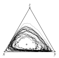
Individual based simulations
The interior fixed point \(\hat x\) is a stable focus of the replicator dynamics. Stochastic fluctuations arise in individual based simulations of populations with a finite size, \(N=1000\). In the absence of mutations, the boundaries are absorbing and even though the interior fixed point is attracting, the population will eventually end up in one of the absorbing homogenous states with all rock, all paper or all scissors.

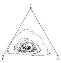
Individual based simulations, with mutations
The interior fixed point \(\hat x\) of the replicator dynamics is an unstable focus. Even without stochasticity all trajectories spiral away from \(\hat x\) towards the boundary of the simplex \(S_3\). However, due to mutations, the boundary is repelling, which results in a stochastic analog of a stable limit cycle. Larger mutation rates increasingly limit the range of values that can be attained by the mean frequencies of the three strategies. In particular, in the limit \(\mu\to1\) the game payoffs no longer affect the dynamics and the mean of all three strategies is simply \(1/3\).
From finite to infinite populations

In unstructured, finite populations of constant size, \(N\), consisting of \(d\) distinct strategic types and with a mutation rate, \(\mu\), evolutionary changes can be described by the following class of birth-death processes: In each time step, one individual of type \(j\) produces a single offspring and displaces another randomly selected individual of type \(k\). With probability \(1-\mu\), no mutation occurs and \(j\) produces an offspring of the same type. But with probability \(\mu\), the offspring of an individual of type \(i\) (\(i\neq j\)) mutates into a type \(j\) individual. This results in two distinct ways to increase the number of \(j\) types by one at the expense of decreasing the number of \(k\) types by one, hence keeping the population size constant. Biologically, keeping \(N\) constant implies that the population has reached a stable ecological equilibrium and assumes that this equilibrium remains unaffected by trait frequencies. The probability for the event of replacing a type \(k\) individual with a type \(j\) individual is denoted by \(T_{kj}\) and is a function of the state of the population \(\mathbf X=(X_1, X_2, \ldots X_d)\), with \(X_n\) indicating the number of individuals of type \(n\) such that \(\textstyle\sum_{n=1}^d X_n = N\).
For such processes we can easily derive a Master equation:
\begin{equation*} P^{\tau+1}({\mathbf X}) = P^{\tau}({\mathbf X})+\!\sum_{j,k=1}^d\! P^{\tau}({\mathbf X}_j^k) T_{kj}({\mathbf X}_j^k)-P^{\tau}({\mathbf X})\ T_{jk}({\mathbf X})) \end{equation*}
where \(P^\tau({\mathbf X})\) denotes the probability of being in state \(\mathbf X\) at time \(\tau\) and \({\mathbf X}_j^k=(X_1, \ldots X_j-1, \ldots X_k+1, \ldots X_d)\) represents a state adjacent to \(\mathbf X\). For large but finite \(N\) the Kramers-Moyal expansion yields a convenient approximation in the form of a Fokker-Planck equation:
\begin{align*} \dot \rho({\mathbf x}) = -\sum_{k=1}^{d-1}\frac{\partial}{\partial x_k}\rho({\mathbf x}){\mathcal A}_{k}({\mathbf x})+\frac12\sum_{j,k=1}^{d-1}\frac{\partial^2}{\partial x_k\partial x_j}\rho({\mathbf x}){\mathcal B}_{jk}({\mathbf x}) \end{align*}
where \({\mathbf x} = {\mathbf X}/N\) represents the state of the population in terms of frequencies of the different strategic types and \(\rho({\mathbf x})\) is the probability density in state \(\mathbf x\). The drift vector \({\mathcal A}_{k}({\mathbf x})\) is given by
\begin{align*} {\mathcal A}_{k}({\mathbf x}) = \sum_{j=1}^{d} \Big(T_{j k}({\mathbf x}) - T_{k j}({\mathbf x}) \Big) = -1+\sum_{j=1}^{d} T_{j k}({\mathbf x}) \end{align*}
For the second equality we have used \(\textstyle\sum_{j=1}^d T_{kj}({\boldsymbol x})=1\), which simply states that a \(k\)-type individual transitions to some other type (including staying type \(k\)) with probability one. \({\mathcal A}_{k}({\mathbf x})\) is bounded in \([-1, d-1]\) because the \(T_{jk}\) are probabilities.
The diffusion matrix \({\mathcal B}_{jk}({\mathbf x})\) is defined as
\begin{align*} {\mathcal B}_{jk}({\mathbf x}) &= - \frac{1}{N} \left[ T_{j k}({\mathbf x}) + T_{k j}({\mathbf x}) \right] \quad {\rm for} \quad j \neq k \\ {\mathcal B}_{jj}({\mathbf x}) &= \frac{1}{N} \sum_{l=1,l\neq j}^d \Big(T_{j l}({\mathbf x})+T_{l j}({\mathbf x}) \Big) \end{align*}
Note that the diffusion matrix is symmetric, \({\mathcal B}_{jk}({\mathbf x}) = {\mathcal B}_{kj}({\mathbf x})\) and vanishes as \(\sim 1/N\) in the limit \(N\to\infty\).
The noise arising through demographic changes and mutations is uncorrelated in time and hence the Itô calculus can be applied to derive a Langevin equation
\begin{align*} \dot x_k = {\mathcal A}_k({\mathbf x}) + \sum_{j=1}^{d-1} {{\mathcal C}_{kj}({\mathbf x})} \xi_j(t) \end{align*}
where the \(\xi_j(t)\) represent uncorrelated Gaussian white noise with unit variance, \(\langle \xi_k(t) \xi_j(t^\prime) \rangle = \delta_{kj} \delta(t-t^\prime)\). The matrix \({{\mathcal C}({\mathbf x})}\) is defined by \({\mathcal C}^T({\mathbf x}) {\mathcal C}({\mathbf x}) = {\mathcal B}({\mathbf x})\) and its off-diagonal elements are responsible for correlations in the noise of different strategic types. In the limit \(N\to\infty\) the matrix \({\mathcal C}({\mathbf x})\) vanishes with \(\sim 1/\sqrt{N}\) and we recover a deterministic replicator mutator equation.
References
- Traulsen, A., Claussen, J. C. & Hauert, C. (2012) Stochastic differential equations for evolutionary dynamics with demographic noise and mutations. Phys. Rev. E 85 041901 doi: 10.1103/PhysRevE.85.041901.
- Traulsen, A., Claussen, J. C. & Hauert, C. (2006) Coevolutionary dynamics in large, but finite populations. Phys. Rev. E 74 011901 doi: 10.1103/PhysRevE.74.011901.
- Traulsen, A., Claussen, J. C. & Hauert, C. (2005) Coevolutionary Dynamics: From Finite to Infinite Populations. Phys. Rev. Lett. 95 238701 doi: 10.1103/PhysRevLett.95.238701.