2×2 Games: Difference between revisions
No edit summary |
No edit summary |
||
| (4 intermediate revisions by the same user not shown) | |||
| Line 20: | Line 20: | ||
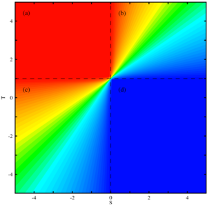
Formally closely related to the prisoner's dilemma is the chicken or hawk-dove game. Actually it changes only the rank ordering of S and P, i.e. the sucker's payoff being more favorable than the punishment: \(T > R > S > P\). Nevertheless, this game addresses quite different biological scenarios of intra-species competition or, in the form of the snowdrift game, explains cooperation under less stringent conditions. The prisoner's dilemma and the snowdrift game are prominent representatives of the more general \(2\times2\) games. Each \(2\times2\) game is characterized and determined by the ranking of the payoffs \(T, R, S, P\) and refers to distinct and substantially different interaction scenarios. All \(2\times2\) games are summarized in the figure on the right. | Formally closely related to the prisoner's dilemma is the chicken or hawk-dove game. Actually it changes only the rank ordering of S and P, i.e. the sucker's payoff being more favorable than the punishment: \(T > R > S > P\). Nevertheless, this game addresses quite different biological scenarios of intra-species competition or, in the form of the snowdrift game, explains cooperation under less stringent conditions. The prisoner's dilemma and the snowdrift game are prominent representatives of the more general \(2\times2\) games. Each \(2\times2\) game is characterized and determined by the ranking of the payoffs \(T, R, S, P\) and refers to distinct and substantially different interaction scenarios. All \(2\times2\) games are summarized in the figure on the right. | ||
{{-}} | {{-}} | ||
== [[2×2 Games / Well-mixed populations|Well-mixed populations]] == | == [[2×2 Games/Well-mixed populations|Well-mixed populations]] == | ||
[[Image:Well-mixed 2x2 Games.png|thumb| | [[Image:Well-mixed 2x2 Games.png|thumb|300px|Equilibrium levels of \(A\) and \(B\) types in well-mixed populations.]] | ||
In this simplest scenario encounters between players are completely random. Such a mean-field approximation is valuable because for the replicator equation the dynamics of \(2\times2\) games can be fully analysed. With \(R=1\) and \(P=0\), this results in four dynamical scenarios: | In this simplest scenario encounters between players are completely random. Such a mean-field approximation is valuable because for the replicator equation the dynamics of \(2\times2\) games can be fully analysed. With \(R=1\) and \(P=0\), this results in four dynamical scenarios: | ||
| Line 31: | Line 30: | ||
# '''bi-stability:''' the states with only \(A\)'s and only \(B\)'s are both stable, i.e. neither rare \(A\)'s nor rare \(B\)'s can invade. The evolutionary end state depends on the initial configuration. This represents a coordination game such as the [[Staghunt game]]. | # '''bi-stability:''' the states with only \(A\)'s and only \(B\)'s are both stable, i.e. neither rare \(A\)'s nor rare \(B\)'s can invade. The evolutionary end state depends on the initial configuration. This represents a coordination game such as the [[Staghunt game]]. | ||
# '''\(A\) dominant:''' This is the complement of the Prisoner's Dilemma and irrespective of the initial configuration the \(A\) types take over the entire population. In the context of cooperation, this situation relates to by-product mutualism. | # '''\(A\) dominant:''' This is the complement of the Prisoner's Dilemma and irrespective of the initial configuration the \(A\) types take over the entire population. In the context of cooperation, this situation relates to by-product mutualism. | ||
{{-}} | {{-}} | ||
== [[2×2 Games / Spatial populations|Spatial populations]] == | == [[2×2 Games/Spatial populations|Spatial populations]] == | ||
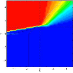
[[Image:Spatial 2x2 Games.png| | [[Image:Spatial 2x2 Games.png|300px|thumb|Equilibrium levels of \(A\) and \(B\) types in spatially extended populations.]] | ||
<!--[[Image:Spatial 2×2 Games (difference).png|200px|thumb|Differences in equilibrium levels of \(A\) and \(B\) types in spatially extended populations as compared to well-mixed populations.]]--> | <!--[[Image:Spatial 2×2 Games (difference).png|200px|thumb|Differences in equilibrium levels of \(A\) and \(B\) types in spatially extended populations as compared to well-mixed populations.]]--> | ||
In structured populations players are arranged on a lattice or network and interact only with their nearest neighbors. The individuals' ability to form clusters can substantially alter the evolutionary outcome. In particular, comparisons with results from well-mixed populations highlight the effects of spatial structure for the four different scenarios of evolutionary dynamics. | In structured populations players are arranged on a lattice or network and interact only with their nearest neighbors. The individuals' ability to form clusters can substantially alter the evolutionary outcome. In particular, comparisons with results from well-mixed populations highlight the effects of spatial structure for the four different scenarios of evolutionary dynamics. | ||
| Line 44: | Line 41: | ||
# '''Bi-stability:''' The pure \(A\) and pure \(B\) state are both stable. This remains unchanged in spatially structured populations but the basins of attraction are very different. In particular, the more efficient \(A\) type has much better chances to take over because it suffices if the threshold density is exceeded locally. | # '''Bi-stability:''' The pure \(A\) and pure \(B\) state are both stable. This remains unchanged in spatially structured populations but the basins of attraction are very different. In particular, the more efficient \(A\) type has much better chances to take over because it suffices if the threshold density is exceeded locally. | ||
# '''\(A\) dominant:''' Generally this is equally true for spatially structured populations. Only if the initial distribution of \(A\)'s is too sparse then they may not be able to expand. | # '''\(A\) dominant:''' Generally this is equally true for spatially structured populations. Only if the initial distribution of \(A\)'s is too sparse then they may not be able to expand. | ||
<!--{{-}} | |||
== [[2×2 Games/Stochastic dynamics|Stochastic dynamics in finite populations]] == | |||
[[Image:Stochastic dynamics - neutral selection, high mutation.png|300px|thumb|Stationary distribution of three strategies \(x, y, z\) in a finite population (\(N=60\)) under neutral selection (\(w=0\)) for mutation rates exceeding the critical mutation rate \(u_c=1/(3+N)\).]] | |||
== [[2×2 Games / Stochastic dynamics|Stochastic dynamics in finite populations]] == | |||
[[Image:Stochastic dynamics - neutral selection, high mutation.png| | |||
In infinite, well-mixed population, the fraction of players can change continuously, as described by the replicator dynamics in [[2×2 Games / Well-mixed populations|well-mixed populations]]. But there are only \(N\) players, then the fraction must change at least by \(1/N\). | In infinite, well-mixed population, the fraction of players can change continuously, as described by the replicator dynamics in [[2×2 Games / Well-mixed populations|well-mixed populations]]. But there are only \(N\) players, then the fraction must change at least by \(1/N\). | ||
| Line 57: | Line 53: | ||
For weak selection, several new features appear in the system: In a bistable situation, one strategy can displace the other. Thus, a new concept of evolutionary stability is necessary. If we consider a single mutant in a population of size \(N\), it will take over the population with probability \(1/N\) without selection, because each individual is equally likely to eventually become the ultimate ancestor. Adding a little amount of selection, a mutant is first disfavored in a bistable situation, but once it has reached a critical fraction, it is favored. The probability that a mutant will take over is a global measure for this process. Interestingly, this probability is larger than \(1/N\) if the mutants become advantageous at a frequency larger than \(1/3\) and smaller then \(1/N\) otherwise, independent of the other details of the underlying game. | For weak selection, several new features appear in the system: In a bistable situation, one strategy can displace the other. Thus, a new concept of evolutionary stability is necessary. If we consider a single mutant in a population of size \(N\), it will take over the population with probability \(1/N\) without selection, because each individual is equally likely to eventually become the ultimate ancestor. Adding a little amount of selection, a mutant is first disfavored in a bistable situation, but once it has reached a critical fraction, it is favored. The probability that a mutant will take over is a global measure for this process. Interestingly, this probability is larger than \(1/N\) if the mutants become advantageous at a frequency larger than \(1/3\) and smaller then \(1/N\) otherwise, independent of the other details of the underlying game. | ||
This result holds for many evolutionary processes under weak selection. Using tools from population genetics, it can be proven that it holds for all processes within the domain of Kingman’s coalescence. | This result holds for many evolutionary processes under weak selection. Using tools from population genetics, it can be proven that it holds for all processes within the domain of Kingman’s coalescence. | ||
--> | |||
{{-}} | {{-}} | ||
| Line 69: | Line 66: | ||
# Traulsen, A., Claussen, J. C. & Hauert, C. (2006) Coevolutionary dynamics in large, but finite populations. ''Phys. Rev. E'' '''74''' 011901 [http://dx.doi.org/10.1103/PhysRevE.74.011901 doi: 10.1103/PhysRevE.74.011901]. | # Traulsen, A., Claussen, J. C. & Hauert, C. (2006) Coevolutionary dynamics in large, but finite populations. ''Phys. Rev. E'' '''74''' 011901 [http://dx.doi.org/10.1103/PhysRevE.74.011901 doi: 10.1103/PhysRevE.74.011901]. | ||
# Traulsen, A., Claussen, J. C. & Hauert, C. (2005) Coevolutionary Dynamics: From Finite to Infinite Populations. ''Phys. Rev. Lett.'' '''95''' 238701 [http://dx.doi.org/10.1103/PhysRevLett.95.238701 doi: 10.1103/PhysRevLett.95.238701]. | # Traulsen, A., Claussen, J. C. & Hauert, C. (2005) Coevolutionary Dynamics: From Finite to Infinite Populations. ''Phys. Rev. Lett.'' '''95''' 238701 [http://dx.doi.org/10.1103/PhysRevLett.95.238701 doi: 10.1103/PhysRevLett.95.238701]. | ||
# Hauert, C. (2001) Fundamental clusters in spatial \(2\times2\) games, ''Proc. R. Soc. Lond. B'' '''268''' 761-769 [http://dx.doi.org/10.1098/rspb.2000.1424 doi: 10.1098/rspb.2000.1424]. | |||
== Acknowledgements == | == Acknowledgements == | ||
Latest revision as of 13:35, 4 August 2024
In behavioral sciences, the essence of various interactions among humans and animals can be modeled by so called \(2\times2\) games. Such games describe pairwise interactions between individuals with two behavioral strategies to choose from. The particular choice of the parametes determines the character of the interaction ranging form cooperation to competition to synchronization. Certainly the most prominent representative is the prisoner's dilemma - a powerful framework to discuss and explain the emergence of altruistic cooperative behavior among unrelated and selfish individuals. Cooperation has long established as a central topic in evolutionary biology because, at least at a first glance, such behavior seems to contradict the principles of darwinian selection. At the same time, cooperation in various repsects must have played a pivotal role in the history of life leading to major transitions such as from genes to chromosomes, from cells to organisms or from individuals to societies. Extensive theoretical studies identified several mechanisms capable of promoting cooperation. The illustration of some of these findings is the main topic of this tutorial.
Prisoner's Dilemma, Snowdrift Game, Chicken & Co.

In a \(2\times2\) game two players simultaneously choose between two options \(A\) or \(B\). Their joint decisions determines the payoff of both players. There are four possible outcomes of the interaction and the respective payoffs can be written as a payoff matrix:
Column player Row player \(\begin{matrix}&A&B\\A&R, R&S, T\\B&T, S&P, P\end{matrix}\)
The first entry in the matrix denotes the payoff to the row player and the second entry the column player's payoff. Therefore, if both players choose \(A\) then each gets \(R\); if the row player chooses \(A\) and the column player \(B\), then the former receives \(S\) and the latter \(T\) and vice versa if column chooses \(A\) and row \(B\); finally, if both choose \(B\), both receive \(P\).
The rank ordering of the four payoff values \(R, S, T, P\) determines the characteristics of the game. Without loss of generality we may assume \(R > P\) (if this does not hold, we simply interchange \(A\) and \(B\)) and normalize the payoff values such that \(R = 1, P = 0\) holds.
Let us first consider the traditional Prisoner's Dilemma: two players simultaneously decide whether to cooperate (\(A\) or \(C\)) or defect (\(B\) or \(D\)). Their joint decisions then determine the payoffs for each player. Mutual cooperation pays a reward \(R\) while mutual defection results in a punishment \(P\). If one player opts for \(D\) and the other for \(C\), then the former obtains the temptation to defect \(T\) and the latter is left with the sucker's payoff \(S\). From the rank ordering of the four payoff values \(T > R > P > S\) follows that a player is better off by defecting, regardless of the opponents decision. Consequentially, rational players always end up with the punishment \(P\) instead of the higher reward for cooperation \(R\) - hence the dilemma. Fortunately there are different mechanisms that allow to overcome this dilemma. This includes repetitions of the interactions with sufficiently high probabilities - the shadow of the future encourages participants to cooperate, i.e. the fear from future retaliation creates incentives to cooperate in the present. Other mechanisms are indirect reciprocity, where individuals carry a reputation, voluntary participation and (spatially) structured populations.
Formally closely related to the prisoner's dilemma is the chicken or hawk-dove game. Actually it changes only the rank ordering of S and P, i.e. the sucker's payoff being more favorable than the punishment: \(T > R > S > P\). Nevertheless, this game addresses quite different biological scenarios of intra-species competition or, in the form of the snowdrift game, explains cooperation under less stringent conditions. The prisoner's dilemma and the snowdrift game are prominent representatives of the more general \(2\times2\) games. Each \(2\times2\) game is characterized and determined by the ranking of the payoffs \(T, R, S, P\) and refers to distinct and substantially different interaction scenarios. All \(2\times2\) games are summarized in the figure on the right.
Well-mixed populations

In this simplest scenario encounters between players are completely random. Such a mean-field approximation is valuable because for the replicator equation the dynamics of \(2\times2\) games can be fully analysed. With \(R=1\) and \(P=0\), this results in four dynamical scenarios:
- \(B\) dominant: Irrespective of the initial configuration the \(B\) type always prevails in the long run. The paradigmatic Prisoner's Dilemma is an example of such dynamics (\(B\) stands for defection).
- co-existence: rare \(A\)'s can invade a resident population of \(B\)'s and vice versa. The evolutionary end state of the population is a mixture both \(A\) and \(B\) types. The most prominent examples of this kind of interactions are given by the Snowdrift game, Chicken game or Hawk-Dove game.
- bi-stability: the states with only \(A\)'s and only \(B\)'s are both stable, i.e. neither rare \(A\)'s nor rare \(B\)'s can invade. The evolutionary end state depends on the initial configuration. This represents a coordination game such as the Staghunt game.
- \(A\) dominant: This is the complement of the Prisoner's Dilemma and irrespective of the initial configuration the \(A\) types take over the entire population. In the context of cooperation, this situation relates to by-product mutualism.
Spatial populations

In structured populations players are arranged on a lattice or network and interact only with their nearest neighbors. The individuals' ability to form clusters can substantially alter the evolutionary outcome. In particular, comparisons with results from well-mixed populations highlight the effects of spatial structure for the four different scenarios of evolutionary dynamics.
- \(B\) dominant: In well-mixed populations \(A\) disappears but in spatially structured populations they may survive in compact clusters. Based on the spatial Prisoner's Dilemma is was concluded that spatial structure is beneficial for cooperation because cluster formation reduces exploitation by defectors.
- Co-existence: As in well-mixed populations both rare \(A\) and rare \(B\) types can invade and the two types co-exist. However, the equilibrium fraction of \(A\) types often tends to be lower than in well-mixed populations. Consequently, in spatially structured populations more frequent escalations of conflicts in the Hawk-Dove game are expected or, similarly, a smaller equilibrium fraction of cooperators in the Snowdrift game. Hence spatial structure may not be as universally beneficial to cooperation as suggested by the Prisoner's Dilemma.
- Bi-stability: The pure \(A\) and pure \(B\) state are both stable. This remains unchanged in spatially structured populations but the basins of attraction are very different. In particular, the more efficient \(A\) type has much better chances to take over because it suffices if the threshold density is exceeded locally.
- \(A\) dominant: Generally this is equally true for spatially structured populations. Only if the initial distribution of \(A\)'s is too sparse then they may not be able to expand.
References

Hauert, C., (2002) Effects of Space in \(2\times2\) Games, Int. J. Bifurcation Chaos 12 1531-1548 doi: 10.1142/S0218127402005273.
The cover shows the equilibrium fraction of cooperators in well-mixed populations as a function of two parameters S, T (see above). Cooperative regions are colored blue and non-cooperative, i.e. regions with prevailing defection, are red. Intermediate fractions of cooperators are shown in light blue, green and yellow (decreasing). The dashed line separates four quadrants with different dynamical characteristics: dominating defection (top left), co-existence (top-right), prevailing cooperation (bottom right) and bi-stability (bottom left). In the last quadrant, the colors indicate the size of the basin of attraction. In blue regions even few cooperators thrive while in reddish regions cooperators prosper only in populations that are already highly cooperative.
Further publications
- Traulsen, A., Claussen, J. C. & Hauert, C. (2006) Coevolutionary dynamics in large, but finite populations. Phys. Rev. E 74 011901 doi: 10.1103/PhysRevE.74.011901.
- Traulsen, A., Claussen, J. C. & Hauert, C. (2005) Coevolutionary Dynamics: From Finite to Infinite Populations. Phys. Rev. Lett. 95 238701 doi: 10.1103/PhysRevLett.95.238701.
- Hauert, C. (2001) Fundamental clusters in spatial \(2\times2\) games, Proc. R. Soc. Lond. B 268 761-769 doi: 10.1098/rspb.2000.1424.
Acknowledgements
For the development of these pages help and advice of the following two people was of particular importance: First, my thanks go to Karl Sigmund for helpful comments on the game theoretical parts and second, my thanks go to Urs Bill for introducing me to the Java language and for his patience and competence in answering my many technical questions. Financial support of the Swiss National Science Foundation is gratefully acknowledged.
