Moran process

Author: Christoph Hauert

The Moran process was named after its inventor, the geneticist P. A. P. Moran, who proposed in 1962 this stochastic process to model evolution in a finite, unstructured (well-mixed) population of constant size \(N\).

Evolutionary dynamics

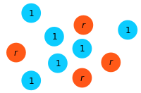
In the simplest case, the population is composed of residents (blue) and mutants (orange):

Setup: The state of the population is given by the number of residents (blue, fitness \(1\)) and mutants (orange, fitness \(r\)).

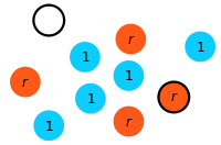
Step 1: At each time step a focal individual is chosen for reproduction with a probability proportional to its fitness (here, a mutant is selected for reproduction).

Step 2: A randomly chosen individual is eliminated (here, a resident is selected for death).

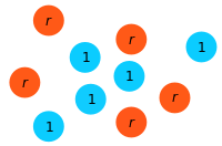
Step 3: The offspring replaces the eliminated individual.

This process is repeated until either one of the two absorbing states is reached: a homogeneous state of either all residents (mutant went extinct) or all mutants (resident displaced). No other stable equilibrium state is possible. Whenever an absorbing state is reached, mutants (residents) are said to have reached fixation. The corresponding fixation probability and fixation time are important markers to characterize the evolutionary process. The Moran process represents a specific balance between selection and drift: advantageous mutations have a certain chance - but no guarantee - of fixation, whereas disadvantageous mutants are likely - but again, no guarantee - to become extinct.

Fixation probability

In unstructured populations the state of the population is fully determined by the number of mutants \(i\), which changes at most by \(\pm 1\) in every time step of the Moran process. With probability \(T_i^+\) the number of mutants increases from \(i\) to \(i+1\), with probability \(T_i^-\) it decreases to \(i-1\) and with probability \(T_i^0=1-T_i^+-T_i^-\) the number of mutants remains unchanged: \begin{align} \qquad T_i^+ &= \frac{i\cdot r}{i\cdot r+(N-i)}\cdot\frac{N-i}N\\ \qquad T_i^- &= \frac{N-i}{i\cdot r+(N-i)}\cdot\frac iN . \end{align} The first factor of \(T_i^+\) (\(T_i^-\)) indicates the probability that a mutant (resident) is chosen for reproduction and the second factor denotes the probability that the offspring replaces a resident (mutant). Note that the ratio of the transition probabilities \(T_i^+/T_i^- = r\) is independent of the number of mutants in the population. This leads to a simple recursive formula for the fixation probability \(\rho_i\) of the mutant in a population with \(i\) mutants: \begin{align} \label{eq:recursive} \qquad\rho_i = \frac r{1+r}\ \rho_{i-1}+\frac 1{1+r}\ \rho_{i+1}.\tag{1} \end{align} Thus, the dynamics corresponds to a biased random walk with absorbing boundaries. Eq. \ref{eq:recursive} represents a homogeneous second order recursion, which can be solved through various means. It is easy to verify that \(\rho_i = 1\) and \(\rho_i = 1/{r^i}\) are two particular solutions. Thus the general solution is a linear combination of the two: \(\rho_i= C_1 + C_2/r^i\). The absorbing boundaries additionally require \(\rho_0=0\) and \(\rho_N=1\), which determine the constants \(C_1,C_2\). The fixation probability of a single mutant \(\rho_1\) then becomes \begin{align} \label{eq:rho1} \qquad\rho_1 = \frac{\displaystyle 1-\frac1r}{\displaystyle 1-\frac1{r^N}}.\tag{2} \end{align} Note that Eq. \ref{eq:rho1} is not defined for the neutral case with \(r=1\). Instead of considering the limit \(r\to1\), it is easy to see that a neutral mutant has a fixation probability of \(\rho_1=1/N\): eventually the entire population will have a single common ancestor but in terms of fitness mutants and residents are indistinguishable and so every member of the population has equal chances to be the chosen one. Evolution is said to favor a mutant if the fixation probability of the mutant exceeds the fixation probability of a neutral mutant, \(\rho_1 >1/N\). In the case that mutations are rare events \(\rho_1\) is of particular interest because the mutant will either have fixated or vanished before the next mutation arises.

In the limit of infinite populations, \(N\to\infty\), the fixation probability for advantageous mutants, \(r>1\), simplifies to \begin{align} \label{eq:rho1inf} \qquad\rho_1 = 1-\frac1r, \end{align} while the fixation probability of disadvantageous mutants, \(r<1\), converges to zero. Even a mutant with double the fitness has only a \(50\%\) chance to fixate. This is in stark contrast to the deterministic dynamics of the replicator equation where any mutant with merely the slightest fitness advantage eventually reaches fixation with certainty.

Celebrated results by the population geneticists Maruyama (1970) and Slatkin (1981) conjecture that fixation probabilities are unaffected by population structures, see Spatial Moran process. Indeed this turns out to be true for a large class of population structures, the Moran graphs but not in general. Instead, some population structures exhibit the intriguing properties that they act as Evolutionary amplifiers, which amplify selection and suppress random drift such that beneficial mutants have a higher chance to fixate as compared to the original Moran process, or as Evolutionary suppressors, which suppress selection and enhance random drift such that beneficial mutants have a lower chance to fixate, again compared to the original Moran process.

References

1. Moran, P. A. P. (1962) Random processes in genetics Proc. Cambridge Phil. Soc. 54 60-71.
2. Maruyama, T. (1974) A Simple Proof that Certain Quantities are Independent of the Geographical Structure of Population Theor. Pop. Biol. 5 148-154.
3. Slatkin, M. (1981) Fixation probabilities and fixation times in a subdivided population Evolution 35 477-488.