Stochastic dynamics in finite populations
In infinite, well-mixed population, the fraction of players can change continuously, as described by the replicator dynamics in well-mixed populations. But in finite populations of size [math]\displaystyle{ N }[/math], the fraction must change at least by [math]\displaystyle{ 1/N }[/math].
In this case microscopic probabilities have to defined that describe how a player switches strategy, as in spatial evolutionary games. There are many ways to define such microscopic evolutionary process. In each of them, strategies that lead to higher payoffs are more likely to spread in the population. For example, two players can be chosen at random to compare their payoffs. The probability that a player adopts the strategy of the other player can be a linear function of the payoff difference. If only better strategies are adopted, the direction of the dynamics becomes deterministic in 2×2 games. But if also worse strategies are sometimes adopted with a small probability, then even a dominant strategy will only take over the population with a certain probability. This approach provides a natural connection between evolutionary game theory and theoretical population genetics, where such probabilities are routinely studied.
Besides the game, two parameters describe the dynamics: The population size [math]\displaystyle{ N }[/math] and the intensity of selection [math]\displaystyle{ w }[/math], which measures how much the adoption of someone else’s strategy depends on the payoffs. If the product of [math]\displaystyle{ w }[/math] and [math]\displaystyle{ N }[/math] is small, one speaks of weak selection and the dynamics is a small correction to random drift. If the product is large, then a deterministic replicator equation is recovered from finite population dynamics.
For weak selection, several new features appear in the system: In a bistable situation, one strategy can displace the other. Thus, a new concept of evolutionary stability is necessary. If we consider a single mutant in a population of size [math]\displaystyle{ N }[/math], it will take over the population with probability [math]\displaystyle{ 1/N }[/math] without selection, because each individual is equally likely to eventually become the ultimate ancestor. Adding a little amount of selection, a mutant is first disfavored in a bistable situation, but once it has reached a critical fraction, it is favored. The probability that a mutant will take over is a global measure for this process. Interestingly, this probability is larger than [math]\displaystyle{ 1/N }[/math] if the mutants become advantageous at a frequency larger than [math]\displaystyle{ 1/3 }[/math] and smaller then [math]\displaystyle{ 1/N }[/math] otherwise, independent of the other details of the underlying game. This result holds for many evolutionary processes under weak selection. Using tools from population genetics, it can be proven that it holds for all processes within the domain of Kingman’s coalescence.
Rock-Paper-Scissors game

Payoff matrix: [math]\displaystyle{ \begin{matrix}~&\begin{matrix}\ \ R\quad & S\quad & P\quad\end{matrix} \\ \begin{matrix}R\\S\\P\end{matrix}& \begin{pmatrix}0 & \frac{s}{2} & -1 \\ -1 & 0 & 2+s \\ \frac{1+s}{3} & -1 & 0\end{pmatrix}\end{matrix} }[/math]
Fixed point: [math]\displaystyle{ \hat{\mathbf x} = \left(\frac12,\frac13,\frac16\right) }[/math]
Deterministic Dynamics
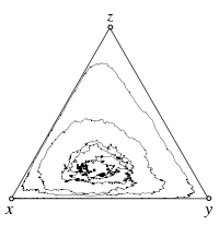
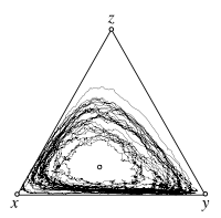
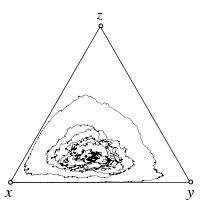
Stochastic Dynamics
Individual Based Simulations
From finite to infinite populations

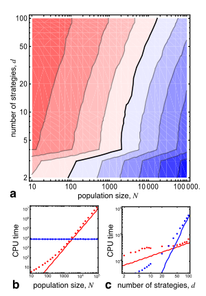
In unstructured, finite populations of constant size, [math]\displaystyle{ N }[/math], consisting of [math]\displaystyle{ d }[/math] distinct strategic types and with a mutation rate, [math]\displaystyle{ \mu }[/math], evolutionary changes can be described by the following class of birth-death processes: In each time step, one individual of type [math]\displaystyle{ j }[/math] produces a single offspring and displaces another randomly selected individual of type [math]\displaystyle{ k }[/math]. With probability [math]\displaystyle{ 1-\mu }[/math], no mutation occurs and [math]\displaystyle{ j }[/math] produces an offspring of the same type. But with probability [math]\displaystyle{ \mu }[/math], the offspring of an individual of type [math]\displaystyle{ i }[/math] ([math]\displaystyle{ i\neq j }[/math]) mutates into a type [math]\displaystyle{ j }[/math] individual. This results in two distinct ways to increase the number of [math]\displaystyle{ j }[/math] types by one at the expense of decreasing the number of [math]\displaystyle{ k }[/math] types by one, hence keeping the population size constant. Biologically, keeping [math]\displaystyle{ N }[/math] constant implies that the population has reached a stable ecological equilibrium and assumes that this equilibrium remains unaffected by trait frequencies. The probability for the event of replacing a type [math]\displaystyle{ k }[/math] individual with a type [math]\displaystyle{ j }[/math] individual is denoted by [math]\displaystyle{ T_{kj} }[/math] and is a function of the state of the population [math]\displaystyle{ \mathbf X=(X_1, X_2, \ldots X_d) }[/math], with [math]\displaystyle{ X_n }[/math] indicating the number of individuals of type [math]\displaystyle{ n }[/math] such that [math]\displaystyle{ \textstyle\sum_{n=1}^d X_n = N }[/math].
For such processes we can easily derive a Master equation:
- [math]\displaystyle{ P^{\tau+1}({\mathbf X}) = P^{\tau}({\mathbf X})+\!\sum_{j,k=1}^d\! P^{\tau}({\mathbf X}_j^k) T_{kj}({\mathbf X}_j^k)-P^{\tau}({\mathbf X})\ T_{jk}({\mathbf X})) }[/math]
where [math]\displaystyle{ P^\tau({\mathbf X}) }[/math] denotes the probability of being in state [math]\displaystyle{ \mathbf X }[/math] at time [math]\displaystyle{ \tau }[/math] and [math]\displaystyle{ {\mathbf X}_j^k=(X_1, \ldots X_j-1, \ldots X_k+1, \ldots X_d) }[/math] represents a state adjacent to [math]\displaystyle{ \mathbf X }[/math]. For large but finite [math]\displaystyle{ N }[/math] the Kramers-Moyal expansion yields a convenient approximation in the form of a Fokker-Planck equation:
- [math]\displaystyle{ \dot \rho({\mathbf x}) = -\sum_{k=1}^{d-1}\frac{\partial}{\partial x_k}\rho({\mathbf x}){\mathcal A}_{k}({\mathbf x})+\frac12\sum_{j,k=1}^{d-1}\frac{\partial^2}{\partial x_k\partial x_j}\rho({\mathbf x}){\mathcal B}_{jk}({\mathbf x}) }[/math]
where [math]\displaystyle{ {\mathbf x} = {\mathbf X}/N }[/math] represents the state of the population in terms of frequencies of the different strategic types and [math]\displaystyle{ \rho({\mathbf x}) }[/math] is the probability density in state [math]\displaystyle{ \mathbf x }[/math]. The drift vector [math]\displaystyle{ {\mathcal A}_{k}({\mathbf x}) }[/math] is given by
- [math]\displaystyle{ {\mathcal A}_{k}({\mathbf x}) = \sum_{j=1}^{d} \Big(T_{j k}({\mathbf x}) - T_{k j}({\mathbf x}) \Big) = -1+\sum_{j=1}^{d} T_{j k}({\mathbf x}) }[/math]
For the second equality we have used [math]\displaystyle{ \textstyle\sum_{j=1}^d T_{kj}({\boldsymbol x})=1 }[/math], which simply states that a [math]\displaystyle{ k }[/math]-type individual transitions to some other type (including staying type [math]\displaystyle{ k }[/math]) with probability one. [math]\displaystyle{ {\mathcal A}_{k}({\mathbf x}) }[/math] is bounded in [math]\displaystyle{ [-1, d-1] }[/math] because the [math]\displaystyle{ T_{jk} }[/math] are probabilities.
The diffusion matrix [math]\displaystyle{ {\mathcal B}_{jk}({\mathbf x}) }[/math] is defined as
- [math]\displaystyle{ \begin{align}{\mathcal B}_{jk}({\mathbf x}) &= - \frac{1}{N} \left[ T_{j k}({\mathbf x}) + T_{k j}({\mathbf x}) \right] \quad {\rm for} \quad j \neq k \\ {\mathcal B}_{jj}({\mathbf x}) &= \frac{1}{N} \sum_{l=1,l\neq j}^d \Big(T_{j l}({\mathbf x})+T_{l j}({\mathbf x}) \Big)\end{align} }[/math]
Note that the diffusion matrix is symmetric, [math]\displaystyle{ {\mathcal B}_{jk}({\mathbf x}) = {\mathcal B}_{kj}({\mathbf x}) }[/math] and vanishes as [math]\displaystyle{ \sim 1/N }[/math] in the limit [math]\displaystyle{ N\to\infty }[/math].
The noise arising through demographic changes and mutations is uncorrelated in time and hence the Itô calculus can be applied to derive a Langevin equation
- [math]\displaystyle{ \dot x_k = {\mathcal A}_k({\mathbf x}) + \sum_{j=1}^{d-1} {{\mathcal C}_{kj}({\mathbf x})} \xi_j(t) }[/math]
where the [math]\displaystyle{ \xi_j(t) }[/math] represent uncorrelated Gaussian white noise with unit variance, [math]\displaystyle{ \langle \xi_k(t) \xi_j(t^\prime) \rangle = \delta_{kj} \delta(t-t^\prime) }[/math]. The matrix [math]\displaystyle{ {{\mathcal C}({\mathbf x})} }[/math] is defined by [math]\displaystyle{ {\mathcal C}^T({\mathbf x}) {\mathcal C}({\mathbf x}) = {\mathcal B}({\mathbf x}) }[/math] and its off-diagonal elements are responsible for correlations in the noise of different strategic types. In the limit [math]\displaystyle{ N\to\infty }[/math] the matrix [math]\displaystyle{ {\mathcal C}({\mathbf x}) }[/math] vanishes with [math]\displaystyle{ \sim 1/\sqrt{N} }[/math] and we recover a deterministic replicator mutator equation.
References
- Traulsen, A., Claussen, J. C. & Hauert, C. (2012) Stochastic differential equations for evolutionary dynamics with demographic noise and mutations. Phys. Rev. E in print.
- Traulsen, A., Claussen, J. C. & Hauert, C. (2006) Coevolutionary dynamics in large, but finite populations. Phys. Rev. E 74 011901.
- Traulsen, A., Claussen, J. C. & Hauert, C. (2005) Coevolutionary Dynamics: From Finite to Infinite Populations. Phys. Rev. Lett. 95 238701.


