2×2 Games/Well-mixed populations: Difference between revisions
m moved 2×2 Games / Well-mixed populations to 2×2 Games/Well-mixed populations: attempt to cleanup sub-pages-mess |
No edit summary |
||
| Line 3: | Line 3: | ||
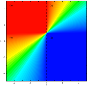
[[Image:Well-mixed 2x2 Games.png|thumb|300px|Four basic evolutionary scenarios of 2×2 Games in the \(S,T\)-plane (with \(R=1, P=0\) ): (a) Dominance of type \(B\) (Prisoner's Dilemma); (b) Stable co-existence of \(A\) and \(B\) types (Snowdrift Game, Hawk-Dove Game, Chicken Game); (c) Bi-stability - the evolutionary outcome depends on the initial configuration (Staghunt Game); (d) Dominance of type \(A\) (Bi-product mutualism). The color code indicates the equilibrium frequency of type \(A\) ranging from low, red to intermediate, green and high, blue. In region (c) the color indicates the size of the basin of attraction of state \(B\).]] | [[Image:Well-mixed 2x2 Games.png|thumb|300px|Four basic evolutionary scenarios of 2×2 Games in the \(S,T\)-plane (with \(R=1, P=0\) ): (a) Dominance of type \(B\) (Prisoner's Dilemma); (b) Stable co-existence of \(A\) and \(B\) types (Snowdrift Game, Hawk-Dove Game, Chicken Game); (c) Bi-stability - the evolutionary outcome depends on the initial configuration (Staghunt Game); (d) Dominance of type \(A\) (Bi-product mutualism). The color code indicates the equilibrium frequency of type \(A\) ranging from low, red to intermediate, green and high, blue. In region (c) the color indicates the size of the basin of attraction of state \(B\).]] | ||
In well-mixed populations the equilibrium fractions of cooperators and defectors are easily calculated using the replicator equation. If \(x\) denotes the fraction of cooperators (and \(1-x\) the fraction of defectors) then their evolutionary fate is given by | In well-mixed populations the equilibrium fractions of cooperators and defectors are easily calculated using the replicator equation. If \(x\) denotes the fraction of cooperators (and \(1-x\) the fraction of defectors) then their evolutionary fate is given by | ||
\begin{align} | |||
\ | \qquad\dot x = \frac{dx}{dt} = x(1-x)(P_A-P_B) | ||
\end{align} | |||
where \(P_A\) and \(P_B\) denote the average payoffs of type \(A\) and type \(B\) players, respectively. The replicator equation basically states that the more successful strategy, i.e. the one with the higher payoff will increase in abundance. The above equation has three equilibria: two trivial ones with \(x_1=0\) and \(x_2=1\) as well as a non-trivial equilibrium for \(P_A=P_B\) which leads to | where \(P_A\) and \(P_B\) denote the average payoffs of type \(A\) and type \(B\) players, respectively. The replicator equation basically states that the more successful strategy, i.e. the one with the higher payoff will increase in abundance. The above equation has three equilibria: two trivial ones with \(x_1=0\) and \(x_2=1\) as well as a non-trivial equilibrium for \(P_A=P_B\) which leads to | ||
\begin{align} | |||
\ | \qquad x_3 = \frac{P-S}{R-S-T+P}. | ||
\end{align} | |||
The replicator equation allows to shift and normalize the payoffs without affecting the dynamics because the performance of cooperators and defectors only depends on the relative payoffs, i.e. on payoff differences. For this reason we can set \(R=1\) and \(P=0\) without loss of generality. Note that the equilibrium \(x_3\) does not necessarily exist, i.e. lie in the interval \([0,1]\). This gives rise to four basic evolutionary scenarios discussed below. | The replicator equation allows to shift and normalize the payoffs without affecting the dynamics because the performance of cooperators and defectors only depends on the relative payoffs, i.e. on payoff differences. For this reason we can set \(R=1\) and \(P=0\) without loss of generality. Note that the equilibrium \(x_3\) does not necessarily exist, i.e. lie in the interval \([0,1]\). This gives rise to four basic evolutionary scenarios discussed below. | ||
Latest revision as of 14:20, 13 October 2023

In well-mixed populations the equilibrium fractions of cooperators and defectors are easily calculated using the replicator equation. If \(x\) denotes the fraction of cooperators (and \(1-x\) the fraction of defectors) then their evolutionary fate is given by \begin{align} \qquad\dot x = \frac{dx}{dt} = x(1-x)(P_A-P_B) \end{align} where \(P_A\) and \(P_B\) denote the average payoffs of type \(A\) and type \(B\) players, respectively. The replicator equation basically states that the more successful strategy, i.e. the one with the higher payoff will increase in abundance. The above equation has three equilibria: two trivial ones with \(x_1=0\) and \(x_2=1\) as well as a non-trivial equilibrium for \(P_A=P_B\) which leads to \begin{align} \qquad x_3 = \frac{P-S}{R-S-T+P}. \end{align}
The replicator equation allows to shift and normalize the payoffs without affecting the dynamics because the performance of cooperators and defectors only depends on the relative payoffs, i.e. on payoff differences. For this reason we can set \(R=1\) and \(P=0\) without loss of generality. Note that the equilibrium \(x_3\) does not necessarily exist, i.e. lie in the interval \([0,1]\). This gives rise to four basic evolutionary scenarios discussed below.
Basic evolutionary scenarios
All of the following examples and suggestions are meant as inspirations for further experimenting with the EvoLudo simulator. Each of following examples starts a lab that demonstrates the particular dynamical scenario. By modifying the parameters the dynamics can be further explored.
| Color code: | Type A | Type B |
|---|

Type A dominates
For \(T<1\) and \(S>0\) the only stable equilibrium is \(x_2=1\) (\(x_1=0\) is unstable and \(x_3\) does not exist). Thus, regardless of the initial configuration of the population type \(A\) will increase and eventually reach fixation.
If \(A\) indicates cooperation and \(B\) defection, then cooperation dominates defection. In biology, this situation refers to by-product mutualism, where cooperative behavior establishes as a by-product of some other activity. For example, the of stotting gazelles is cooperative behavior because it warns their fellows from approaching predators but at the same time it startles predators and displays the individuals strength, which might persuade the predator to go after another individual. The relative costs and benefits of these two aspects of stotting behavior determine whether warning other gazelles occurs only as a by-product.

Type B dominates
Conversely, for \(T>1\) and \(S<0\) the only stable equilibrium is \(x_1=0\) (\(x_2=1\) is unstable and \(x_3\) does not exist). Thus, type \(A\) players eventually disappear irrespective of the initial configuration of the population.
If \(A\) indicates cooperation and \(B\) defection, then defection dominates cooperation. In biology, this situation is represented by the famous Prisoner's Dilemma (for further details see the tutorial on Cooperation in structured populations).

Coexistence
For \(T>1\) and \(S>0\) both trivial equilibria \(x_1, x_2\) are unstable and the equilibrium \(x_3\) must exist and must be stable. In that case, type \(A\) and \(B\) individuals can co-exist.
This situation corresponds to the Snowdrift game, Chicken or Hawk-Dove game used to model cooperation and competition in biology (for further details see the tutorial on Cooperation in structured populations).

Bistability
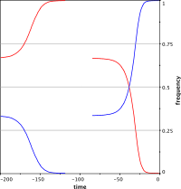
Finally, for \(T<1\) and \(S<0\) both trivial equilibria are stable with an unstable equilibrium \(x_3\) in the interior. Depending on the initial configuration of the population either cooperators or defectors will increase and reach fixation. The position of \(x_3\) determines the basin of attraction of the evolutionary end states of all cooperation or all defection. If the initial fraction of cooperators exceeds \(x_3\) then the \(A\) types prevail but vanish otherwise.
This situation represent a coordination game often referred to as a Staghunt game.
